¹Alfred Wegener Institute, Helmholtz Centre for Polar and Marine Research, Germany

²Department of Civil and Environmental Engineering, King Fahd University of Petroleum and Minerals, Dhahran 31261, Saudi Arabia

³Interdisciplinary Research Center for Construction and Building Materials, KFUPM, Dhahran 31261, Saudi Arabia

⁴Bremerhaven Institute of Nanotechnology, Process Engineering and Energy Technology, University of Applied Sciences, Bremerhaven, Germany

*Corresponding author: Department of Civil and Environmental Engineering, King Fahd University of Petroleum and Minerals, Dhahran 31261, Saudi Arabia; Email: [email protected];  [email protected]

Received Date: December 08, 2023

Publication Date: February 27, 2024

Citation: Olanrewaju OS, et al. (2024). Structural Risk and Reliability Assessment of Offshore Aquaculture Floating System for Seaweed Cultivation. Material Science. 6(1):24.

Copyright: Olanrewaju OS, et al. © (2024). 

ABSTRACT

The materials used for offshore aquaculture floating structures in seaweed farming usually have less durability due to oceanic environmental factors. This affects the production of seaweed and increases the cost of production due to the breakdown of the structures. The floating structure of seaweed farming can be improved by choosing a suitable material based on the material properties such as strength, and safe working load. Structural assessment of the components of floating structures for seaweed farming has been investigated. Past materials used by farmers are reviewed to assess suitable material for offshore structures and the hydrostatic analysis is carried out to determine the pressure and dynamics load that the structures can withstand such as wind and current. Finally, reliability analysis using Fault Tree Analysis is conducted to determine the probability of failure of the structural components based on different events. This study has shown that high-molecular polyethylene is a very suitable material for offshore structures.

Keywords: Offshore aquaculture, Risk, Reliability, Floating structures, Seaweed farming, Hydrostatic, High-molecular polyethylene

INTRODUCTION

Interest in culturing and harvesting seaweed offshore began in Japan roughly four decades ago. The use of seaweed as food has been tracked back to the 4^th century in Japan and the 6^th century in China. As stated by Fisheries and Aquaculture Organizations (FAO), in the Prospect for Seaweed Production in Developing Countries [1], Japan, China, and Korea are the largest consumers of seaweed as food and their requirements provide the basis for the industry that worldwide harvests 6 million tons of wet seaweed per annum with a value of around US$ five billion [2]. The book Seaweed in Agriculture and Horticulture [3] reported that seaweed contains all major and minor plant nutrients, and trace elements; alginic acid; vitamins; auxins; at least two gibberellins; and antibiotics. Therefore, seaweed is also good for health. Seaweed has been used as human food since ancient times [4]. In the past decade, some French research and development institutions have placed considerable effort into the development of edible seaweed products to introduce them to the European diet and market.

Seaweed (or sea vegetables) is a large and diverse group of marine macroalgae that can be found in intertidal coastal regions around the world. Seaweeds can be classified into three broad groups based on the colors brown, red, and green. Botanists refer to these broad groups as Phaeophyceae, Rhodophyceae, and Chlorophyceae, respectively [5-6]. In most of the world, seaweed is farmed using wild harvesting. In the autumn each year, farmers would throw bamboo branches into shallow, shady water, where the spores of the seaweed would be collected. A few weeks later, the seaweed will be moved to the estuary so that the seaweed can absorb more nutrients to grow. Then, the method was improved by using the ‘Hibi’ method, which is the simple rope stretched between bamboo poles. In addition, it is difficult and expensive to increase the size of bamboo rafts to a farm-size scale practiced by most farmers [7-8].

Floating structures have been commonly used and improved from time to time in seaweed industry development [9-10]. However, the design of the offshore structure for seaweed farming is non-durable while the industry is developing rapidly [11]. The project to reduce the cost and maintenance of the system through suitable material selection and de-risking other engineering challenges is being developed. The impact of aquaculture on the environment and the effects of the environment on aquaculture production have become important issues in recent years. The study discusses the following environmental implications associated with the seaweed culture and material selection and ways in which cultivation can be made efficient and ecologically friendly

The offshore floating structure for seaweed farming is non-durable and unsustainable, this leads to an increase in the maintenance costs for the structure. Therefore, to reduce the maintenance cost, the study of the type of material needs to be carried out. The offshore floating structures are not strong enough to withstand the pressure from the ocean environment. This affects the seaweed and increases the maintenance cost. Therefore, a suitable type of material must be chosen to make sure the structure is long-lasting. The traditional offshore floating structures are not stable enough when loading and unloading. The structure cannot withstand the loads that they carry. A strong type of material must be chosen to make sure the structures are stable. Some of the offshore floating structures pollute the farming areas. For example, the use of bamboo sticks is non-durable, therefore it will rot and will pollute the sea areas. The new floating structures and the material will avoid this problem.

METHODOLOGY

The study involves the review of material for very large floating structures. Then, it is followed by an assessment of the structural components, the structural analysis that involves reliability, and hydrostatic analysis.

HYDROSTATIC ANALYSIS

The hydrostatic analysis involves underwater weighing, hydrostatic body composition analysis, and hydro densitometry (mass per unit volume of a body) to provide volume information about the body and its interaction with water. Elastic response analysis involves the use of Archimedes’ principle, to measure the weight of the body outside the water, the weight of the completely immersed body, and the density of the water. This measurement provides important buoyancy information about the body and its response forces in water [12].

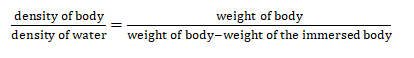                                                                        (1)

The hydrostatic load is obtained by considering several factors such as wind load, sea currents, and wave load in the estimation. To some extent, most solid materials exhibit elastic behavior, but there is a limit to the magnitude of the force and the accompanying deformation. The elastic response can show whether the components of the structure can withstand the load and pressure that is exerted on the structure. The elastic response can be divided into two which are static and dynamic responses analysis. The buoyancy force is determined by:

                                                                                                                                                               

where ρ is the density of the fluid, g is the acceleration due to gravity, and V is the volume of fluid directly above the curved surface. This formula is used to determine the buoyancy force of the components of the structure.

DYNAMIC RESPONSE

Although wind load is dynamic, offshore structures respond to them in a nearly static fashion. However, a dynamic analysis of the unit/installation is indicated when the wind field contains energy at frequencies near the natural frequencies of the unit/installation (fixed or moored to the ocean bottom) [13]. Sustained wind speed is used to determine the global load acting on the unit/installation, and gust speed should be used for the design of individual structural elements.

Wind

The wind will give pressure to any object or body in its path. In this case, before determining the wind force, the mean wind speed must be determined. Mean wind speed can be divided into two factors which are sustained wind speed and wind gust speed. Sustained wind speed is indeed the average wind over a given interval. The common reference height is ten meters. Wind forces are computed using the one-minute mean wind speed, and appropriate formulas and coefficients may be derived from applicable wind tunnel tests. The sustained wind speed is estimated by:

                                                                                                                                    

where u(t) is the mean wind speed at a reference height of 10 m [m/s] = 0.167 m/s, Ct is the wind speed averaging time factor, u(tr) is the reference wind speed [m/s], t is the averaging time [minutes] and tr is the reference time = 10 [minutes].

Wind gusts occur when the peak wind speed reaches at least 16 knots and the variation in wind speed between the peaks and lulls is at least 9 knots. The greatest three-second mean wind speed, expected to occur over a return period of 100 years, is referred to as the wind gust speed, uG. This wind gust speed is to be used for the determination of local loads. The wind gust speed is related to the sustained wind speed as follows:

                                                                                                                                    

where uG is wind gust speed and uS is sustained wind speed. Combining Eq. (3) and Eq. (4), the wind speed is determined by:

                                                                                                                                       

From the calculation, the average maximum wind speed v(t) for the East Coast is obtained as shown in Figure 1 and Table 1.

Table 1: Average Maximum Speed for the East Coast.

Time (second)	Time (Minute)	V(t)
3	0.05	1.43
5	0.080	1.39
10	0.17	1.35
20	0.30	1.28
30	0.50	1.26
60	1.00	1.20
120	2.00	1.16
300	5.00	1.07
600	10.00	1.00
3600	60.00	0.94

 

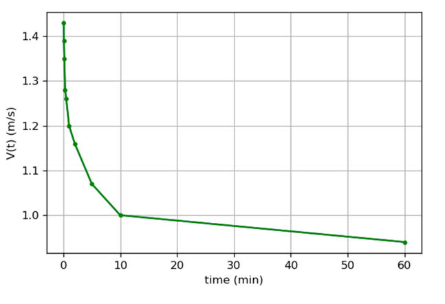
Figure 1: Average Maximum Speed versus Time

Near Surface Current

Near-surface, the current is a wind/wave-generated current. For near-surface currents, the design velocity may be estimated as follows.

where uw(z) is the near-surface current velocity [m/s], k(z) is the factor depending linearly on the vertical coordinate, z, and can be calculated easily as follows.

k(z) = 0. 01 for z = 0 m

       = 0 for z ≥ –15 m, to be obtained by linear interpolation for 0 > z > –15 m

z is the vertical coordinate axis above mean sea level [m] and uS is the sustained wind speed used for design [m/s] = one-minute mean at z = 10 m.

RELIABILITY ANALYSIS

The assessment of scale reliability is based on the correlations between the individual items or measurements that make up the scale, relative to the variances of the items. A measure of reliability is the measure that one can easily infer a measure or statistic to describe the reliability of an item or scale. Specifically, an index of reliability can be defined in terms of the proportion of true score variability that is captured across subjects or respondents, relative to the total observed variability [14]. Schueremans and Van Gemert [15] proposed the following target failure probability under the action of failure model, the limit state equation of structure is generally expressed as:

where T is residual service life, N is the number of lives put in danger, S is the social criterion factor (preservation value), A is the activity factor, C_F is the economic factor (consequences of failure), and W is the warning factor. The warning factor corresponds to the likelihood that, given failure or recognition of approaching failure, seaweed in this case at risk will be dead. The economic factor reflects cost-benefit considerations. Table 2 shows the annual target probability of failure and acceptability [16] whereas Table 3 shows the annual target reliability index for ultimate limit states [17].

Table 2: Annual Target Probability of Failure and Acceptability

Annual Target Pf			Degree of Acceptability
10-1 - 10-3			Unacceptable
10-4			Control with public expenditure
10-5			Rare, but voluntary risk (e.g., drowning)
10-6			Acceptable (e.g., act of God)
Alternative Measure of Reliability – Reliability Index β
Pf	10-1	10-2	10-3	10-4	10-5	10-6
β	1.28	2.32	3.09	3.71	4.25	4.75

Table 3: Annual Target Reliability Index for the Ultimate Limit States.

Relative Cost of Safety Measure	Minor consequences	Moderate consequences	Large consequences
Large	β=3.1	β=3.3	β=3.7
Normal	β=3.7	β=4.2	β=4.4
Small	β=4.2	β=4.4	β=4.7

QUANTITATIVE RISK ANALYSIS

Quantitative risk analysis (QRA) is a process for assigning a numeric value to the probability of loss based on known risks and available, objective data used to determine potential direct and indirect costs based on values assigned to assets and their risk exposure. Kaplan and Garrick [18] suggested that rational decision-making requires, therefore, a clear and quantitative way of expressing risk so that it can be properly weighed, along with all other costs and benefits, in the decision process. Several methods are used to assess QRA including Event Tree Analysis (ETA), Fault Tree Analysis (FTA), and risk matrix, etc [19]. In this case, the method to calculate risk is FTA. It is used qualitatively to identify the individual scenarios (so-called paths or cut sets) that lead to the top (fault) event, while it is also used quantitatively to estimate the probability (frequency) of that event.

RESULTS AND DISCUSSION

PARAMETRIC STUDY OF MATERIALS USED FOR VERY LARGE FLOATING STRUCTURES

Figure 2 shows the floating structure of seaweed farming. Autocad software is used to design the floating structure. The dimension of seaweed farming is 100 meters × 100 meters, and it consists of four big buoys at the corner and small buoys at an interval distance of around 5 meters. The size of big buoys is 0.6 meters in diameter and the diameter size of about 0.17 meters for small buoys. From the calculations that have been made, those sizes of buoys are suitable to withstand environmental loads and also dead loads from seaweed itself [20-21]. Figure 3 shows the drawing of the floating structure seen from the top view and the separator lines are seen from the diagram.

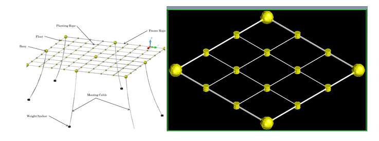
Figure 2: Floating Structure of Seaweed Farming, Figure 3: Drawing of Floating Structure

FUNCTIONALITY REQUIREMENT

Typically, functional requirements will specify a behavior or function of what the system of floating structure should do. In this case, the offshore aquaculture floating structure of seaweed farming involves the design of the mooring system used to anchor and provide station-keeping for the seaweed plantation platform to the seafloor to prevent tangling to the seaweed and excessive movement of the platform [22].

In the past, farmers used bamboo sticks for their system which are not durable and cannot withstand high pressure from the environment even though it is cheap and easy to get. Today, the farming system has improved with new technology that uses floating structures from the offshore industry. However, sometimes, the materials used are not durable and it can increase the cost of farming. To solve this problem, the purposes of using high-quality and reliable materials are important to gain more benefits from seaweed farming.

STANDARD REQUIREMENT

In this case, some research and observation have been made in choosing good materials for offshore aquaculture floating structures for seaweed farming. Table 4 shows some research and observations that have been made among High-Density Polyethylene (HMPE), Polypropylene, and Polyester rope in the aspects of strength, UV resistance, strain, specific gravity rigidity, and abrasion resistance. Table 5 shows the score of each material by comparing its characteristics. This is a 3-point score with 1 (poor), 2 (moderate), and 3 (good). It is almost like PCC (pairwise comparison chart). The mark is based on the advantages each of the materials possesses. In this case, HMPE gets the highest mark which is 15 followed by Polyester with 13 and Polypropylene with 12. Due to the highest score in strength rigidity, and abrasion resistance, HMPE is considered to be the best material. Thus, it is the best material for the important part of the floating structure which is the frame line due to its responsibility to carry out important functions for the structure. For the separator line, polyester is used to lower the cost of the construction caused by the function which is not as important as the frame line and planting line.

Table 4: The Properties of Chosen Materials for Certain Aspects.

Rope/Characteristic	HMPE	Polypropylene	Polyester
Strength	Excellent	Good	Good
UV Resistance	Stable	Poor	Excellent
Strain	Low	High	Low
Specific Gravity	0.98	0.91	1.38
Rigidity	High	Moderate	Moderate
Abrasion Resistance	High	Moderate	High

Table 5: Grading of Chosen Materials for Certain Aspects.

Rope/Characteristic	HMPE	Polypropylene	Polyester
Strength	3	1	2
UV Resistance	2	1	3
Strain	2	3	2
Specific Gravity	2	3	1
Rigidity	3	2	2
Abrasion Resistance	3	2	3
Total Score	15	12	13

For buoy material, many types of buoys are made of polyethylene because of high demand from all types of applications and because it is easy to get from suppliers. In this case, UV stabilized polyethylene buoy is chosen due to a lot of usages in the offshore industry and is very durable. Some of their advantages are listed as follows and this is why UV-stabilized polyethylene is highly recommended for offshore floating structures: high chemical and corrosion resistance, excellent buoyancy characteristics, excellent strength, ability to withstand pressure from the environment, and requires minimal maintenance.

ASSESSMENT OF STRUCTURAL COMPONENTS

A risk assessment to identify potential hazards and analyze what could happen if a hazard occurs is conducted. In this section, the potential risks and the measures to control are discussed for the frame line, planting line, buoy, rope, and separator line. The score for each structural component is measured based on their functions to the structure. The score of 6 for the frame line and separator line shows that their risk is more than medium. For the planting line, a score of 7 is given which is a category that must be taken seriously because their role is important which is to withstand pressure from environmental load and also dead load from the seaweed. For the buoy, a score of 8 is given which is higher than the planting line and the frame line because it needs to accommodate major loads from the structure. The highest score is given to the rope which is 9 because it is a major component that determines the durability of the structure.

STRUCTURAL ANALYSIS

Structural analysis is conducted to determine the effects of loads on physical structures and their components. Structural analysis incorporates material science and applied mathematics to compute structural deformations, internal forces, stresses, support reactions, accelerations, and stability. The results of the analysis are used to verify the fitness for use, often with physical tests.

HYDROSTATIC ANALYSIS

A hydrostatic analysis is a study of incompressible fluids at rest. It encompasses the study of the conditions under which fluids are at rest in stable equilibrium as opposed to fluid dynamics, the study of fluids in motion [23]. Hydrostatic is categorized as a part of fluid statics, which is the study of all fluids, incompressible or not, at rest. The hydrostatic analysis is divided into two parts that are elastic response and dynamic or transient response. In static response, the system is assumed to be in equilibrium or there is no force exerted on the system. Therefore, it is said to be static because there is no movement of the body. For the dynamic response, the system is assumed to be in the state of forces exerted on the system such as wind, wave, and current.

Static analysis is a term for simplified analysis wherein the effect of an immediate change on a system is calculated without respect to the longer-term response of the system to that change. Table 6 shows the buoy specification. Table 7 is the summary of Table 6. The size and weight of the buoy affect the buoyancy and density of the buoy. The less dense the buoy, the more the buoy will float and can withstand the load.

Any arbitrary shape that is immersed, partly or fully, in a fluid will experience the action of a net force in the opposite direction of the local pressure gradient. Table 8 shows the volume of the water displaced affects the force exerted on the buoyancy structure. The results from the calculation of the rope and seaweed are shown in Table 9, Table 10, Table 11, and Table 12.

Table 6: Buoy Specification.

No.	Density of Seawater (kg/m3)	WOB (kg)	WTB (kg)	Diameter (m)	Size (volume=m3)	Up-thrust (kg/m3)	G (m/s-2)	DOB (kg/m3)
1	1.025	0.63	0.588	0.20	4.189x10-3	0.042	9.80	1.098
2	1.025	0.76	0.7342	0.17	2.572 x10-3	0.026	9.80	0.88
3	1.025	0.87	0.8213	0.21	4.849 x10-3	0.049	9.80	1.086
4	1.025	0.97	0.878	0.20	4.189 x10-3	0.042	9.80	1.132
5	1.025	1.2	1.1273	0.24	7.238 x10-3	0.073	9.80	1.091
6	1.025	1.48	1.438	0.20	4.189 x10-3	0.042	9.80	1.099

where WOB is the weight of the body (kg), WIB is the weight of the immersed body (kg), Size is the size of the buoy in volume (), and Up-thrust is the upward force that a liquid or gas exerts on a body floating on it, G is the gravity of earth (m/sˉ²), and DOB is the density of body (kg/m³).

Table 7: Density of Buoy based on Weight and Size.

Size of Buoy (m3)	Weight of Buoy (kg)	Density of Buoy (kg/m3)
4.189x10-3	0.63	1.098
2.572 x10-3	0.76	0.88
4.849 x10-3	0.87	1.086
4.184 x10-3	0.97	1.132
7.238 x10-3	1.20	1.091
4.189 x10-3	1.48	1.099

Table 8: Buoyancy Force of Buoy in Seawater.

ρ (kg/m3)	G (m/s2)	V (m3)	F (N)
1.025	9.80	4.189x10-3	0.042
1.025	9.80	2.572 x10-3	0.026
1.025	9.80	4.849 x10-3	0.049
1.025	9.80	4.184 x10-3	0.042
1.025	9.80	7.238 x10-3	0.073
1.025	9.80	4.189 x10-3	0.042

Table 9: Rope Specification.

No	DOS	WOR	WOR2	Diameter (m)	Size (volume= m3)	MBF	G
1	1.025	4.2	1.68	0.006	2.83x10-3	4.48	9.8
2	1.025	7.5	3	0.008	0.02	10.4	9.8
3	1.025	11	4.4	0.01	0.031	15.3	9.8
4	1.025	18.47	7.388	0.018	0.1	47.2	9.8
5	1.025	22.73	9.092	0.02	0.13	56.9	9.8
6	1.025	32.3	12.92	0.024	0.18	79.7	9.8

where DOS is the density of seawater, WOR is the weight of rope in kg for 250 m, WOR2 is the weight of rope for 100 m, MBF is the minimum breaking force (kN), and Diameter is the diameter of rope (meter).

Table 10: Buoyancy Force of Rope in Seawater.

ρ (kg/m3)	G (m/s2)	V (m3)	F (N)
1.025	9.80	2.83x10-3	0.028
1.025	9.80	0.02	0.2009
1.025	9.80	0.031	0.311395
1.025	9.80	0.1	1.0045
1.025	9.80	0.13	1.30585
1.025	9.80	0.18	1.8081

Table 11: Seaweed Specification.

DOS	WOS	WIS	Length	Thickness	CD	Diameter (m)	Size (volume= m3)	G
1.025	0.41	0.001	0.26	0.002	0.16	0.02	1.664x10-6	9.8

where WOS is the weight of seaweed in the air (kg), WIS is the weight of immersed seaweed (kg), Length is the length of seaweed, Diameter is the diameter of seaweed (meter), Size (volume=m³) is the size of seaweed, Thickness is the thickness of seaweed, and CD is the drag coefficient of seaweed.

Table 12: Buoyancy Force of Seaweed in Seawater.

ρ (kg/m3)	G (m/s2)	V (m3)	F (N)
1.025	9.8	1.664x10-6	1.67x10-5

For the components of the structure which are rope, buoy, and seaweed, their buoyancy forces are determined and compiled together to get the total force that the floating structure can carry. For the rope, two different sizes of rope are chosen for the frame line and separator line, whereas for the buoys, large-size buoys are used for the corner buoy, and small-size buoys are used for the middle buoys. As shown in Table 13, the total load that the structure can carry is 29.426N if no additional forces are acting on the structure.

Table 13: Total Forces for the Whole Structure.

Components	Name	Weight	Length	Quantity	Total W	F	Total F
1	L. buoy	1.1	0.6	4	4.4	0.073	0.292
2	S. buoy	0.73	0.17	400	292	0.026	10.4
3	Frame rope	12.92	100	4	51.68	1.8	7.2
4	S. rope	1.68	100	400	672	0.028	11.2
5	Seaweed	0.001	0.26	20000	20	1.67x10-5	0.334
				Total W	1040.08	Total F	29.426

where L. buoy is a large buoy, S.buoy is a small buoy, the rope is a separator, Weight is the weight of components (kg), Length is the length of components (meter), and Quantity is the quantity needed for the whole structure, Total W is the total weight of components for quantity needed, F is the buoyancy force of the components, Total F is the total buoyancy force of components for quantity needed, Total w is the total weight of the structure, and Total F is the total force of the structure.

DYNAMIC RESPONSE

The dynamic response is the time-varying motion of a structure subjected to a given input dynamic force. For example, for a space vehicle that is exposed to the side-acting wind during flight, the dynamic response would consist of a rigid body rotation of the vehicle plus a bending deformation, both changing with time. Ultimately, knowing the dynamic response of the system is essential if the system is influenced by the behavior. There are three components for the dynamic load, which are wind, wave, and current. Before analyzing how much the structure can withstand the loads from the surroundings, the force from each load must be calculated.

Wind force

The wind force is the pressure exerted by the wind on the structure. It is the total force exerted upon a structure by the wind. Table 14 shows wind speed averaging time factors [24] and Table 15 shows mean sustained wind speed at a reference height of 10 m. Figure 4 shows sustained wind speed versus time.

Table 14: Wind Speed Averaging Time Factors C_t

Averaging time t (second)	Ct
3	1.249
5	1.225
15	1.173
60	1.108
600	1.000
3600	0.916

Table 15: Mean Sustained Wind Speed at Reference Height of 10 m.

Time (second)	Ct	u(tr) (m/s)	u(t) (m/s)
3	1.249	0.167	0.2086
5	1.225	0.167	0.2046
15	1.173	0.167	0.1959
60	1.108	0.167	0.1850
600	1.000	0.167	0.1670
3600	0.916	0.167	0.1530

 

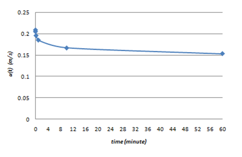
Figure 4: Sustained Wind Speed versus Time.

The wind gust component may be considered as a zero-mean random wind component when superimposed on the constant, average wind component yields the short-term wind speed. A wind gust usually comes in 2-minute intervals and comes quite suddenly and abruptly. There are several different reasons for wind gusts to occur. One of the causes of a wind gust is when there is a sudden shift from high pressure to low pressure. Another cause for a wind gust to occur is the terrain. Wind gusts are more frequent in areas where there are extremely tall trees or man-made infrastructures. The wind in a 3-second gust is appropriate to determine the maximum static wind load on individual members; a 5-second gust is appropriate for maximum total loads on structures whose maximum horizontal dimension is less than 50, and a 15-second gust is appropriate for the maximum total static wind load on larger structures. The one-minute sustained wind is appropriate for total static superstructure wind loads associated with maximum wave forces for structures that respond dynamically to wind excitation but do not require a full dynamic wind analysis. For structures with negligible dynamic response to winds, the one-hour sustained wind is appropriate for total static superstructure wind forces associated with the maximum wave forces. The wind gust speed is calculated as follows.

uG = 1.137. uS

=1.137. 0.167

=0.1895 m/s

Table 16 shows the mean gust wind speed at a reference height of 10 m and Figure 5 shows the gust wind speed versus time.

Table 16: Mean Gust Wind Speed at Reference Height of 10 m.

Time (second)	Ct	u(G) (m/s)	u(t) (m/s)
3	1.249	0.1895	0.2367
5	1.225	0.1895	0.2321
15	1.173	0.1895	0.2223
60	1.108	0.1895	0.2100
600	1.000	0.1895	0.1895
3600	0.916	0.1895	0.17358

 

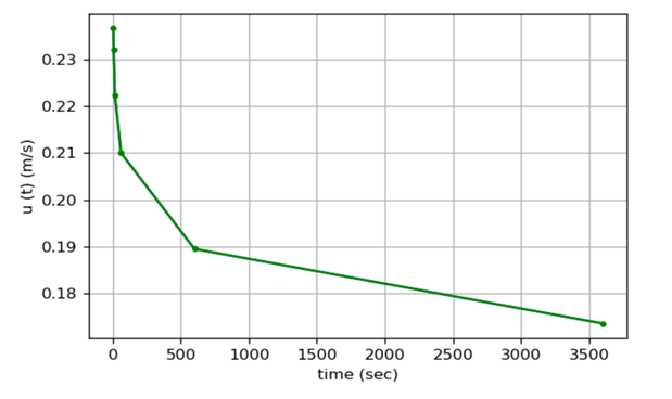
Figure 5: Gust Wind Speed versus Time.

Currents

In this section, ocean currents can be divided into four categories which are near-surface currents, sub-surface currents, sea currents, and currents force. Tables 17 and 18 show the near-surface current velocity for sustained wind speed and gust wind speed, respectively.

Near-surface currents for sustained wind speed

Table 17: Near-surface Current Velocity for Sustained Wind Speed

Time (second)	k(z)	us (m/s)	uw(z) (m/s)
3	0.01	0.2086	0.002086
5	0.01	0.2046	0.002046
15	0.01	0.196	0.00196
60	0.01	0.185	0.00185
600	0.01	0.167	0.00167
3600	0.01	0.153	0.00153

1. Near-surface currents for gust wind speed

Table 18: Near-surface Current Velocity for Gust Wind Speed.

Time (second)	k(z)	uG (m/s)	uw(z) (m/s)
3	0.01	0.237	0.00237
5	0.01	0.232	0.00232
15	0.01	0.222	0.00222
60	0.01	0.21	0.0021
600	0.01	0.19	0.0019
3600	0.01	0.174	0.00174

RELIABILITY ANALYSIS

Reliability analysis is used to construct reliable measurement scales to evaluate the reliability of the floating structure of seaweed farming [25]. Based on the risk assessment of the structural members, Failure Modes, and Effect Analysis (FMEA) is conducted. The Risk Priority Number (RPN) number in Table 19 is obtained from Table 20. From the result, it can be concluded that the risk ratings for all the components are exceeded or equal to 42. Therefore, actions should be taken to cease the work until appropriate additional control measures are implemented.

Table 19: Severity Number for Components

Potential Risk	Frame Line	Planting Line	Buoy	Rope	Separator Line	RPN Number
	Severity Number (1-10)
Break Fatigue Unsuitable frame design Inadequate rope	7				7	252
The size and buoyancy			9	9		576
Loose Stack rope Too heavy Cannot float Arrangement		9				441
Fatigue Not durable Size and weight of the rope Suitable material for the rope Strength of the rope				5		405

Table 20: Risk Matrix.

                       

FAULT TREE ANALYSIS (FTA)

The application of a Fault Tree may be illustrated by considering the probability of failure of the floating system such as the break of the rope or damage to the structure by all possibilities and constructing a tree with AND and OR logic gates. The failures of the structure: For qualitative analysis, by using the property of the Boolean algebra, it is possible to establish the combination of basic (components) failures that can lead to the top (undesirable) event when occurring simultaneously. These combinations are so-called "minimal cut sets" and can be derived from the logical equation represented by the Fault Tree. Considering the Fault Tree, eleven scenarios can be extracted:

1. Earthquake                                            AND    floating structures
2. Tsunami                                 AND    floating structures
3. Wave too high                       AND    floating structures
4. Wind too tight                       AND    floating structures
5. Current too high                                   AND    floating structures
6. Wave speed too high                            AND    floating structures
7. Current speed too high        AND        floating structures
8. Wind speed too fast                              AND    floating structures
9. Loads of seaweed too heavy AND    floating structures
10. Strength of rope loose          AND        floating structures
11. Break of rope loose                               AND        floating structures

These 11 minimal cut sets are in the first approach equivalent. However, a common cause failure analysis could show, for example, that the "wave speed too high" increases the probability of failure of "floating structures" because the wave is too high from all directions. It can be concluded that the 4th cut set is more likely than the others.

For semi-quantitative analysis, it is the second step which consists of calculating the probability of occurrence of each scenario. By ascribing probabilities to each basic event, Table 21 is obtained.

Table 21: Probability of Failure and Cut Sets.

Event	Probability	Structures	Pf	Pf
1	0.1	0.01	0.001	1x10-3
2	0.1	0.01	0.001	1x10-3
3	0.01	0.01	0.0001	1x10-4
4	0.01	0.01	0.0001	1x10-4
5	0.001	0.01	0.00001	1x10-5
6	0.001	0.01	0.00001	1x10-5
7	0.001	0.01	0.00001	1x10-5
8	0.001	0.01	0.00001	1x10-5
9	0.001	0.01	0.000001	1x10-6
10	0.001	0.01	0.000001	1x10-6
11	0.001	0.01	0.000001	1x10-6

Total = 0.002243 = 2.243x10^-3

where P_f = probability of failure, Event 1= Earthquake, Event 2 = Tsunami, Event 3 = Wave too high,

 4 = Wind too tight, Event 5 = Current too high, Event 6 = Wave speed too high, Event 7 = Current speed too high, Event 8   = Wind speed too fast, Event 9 = Loads of seaweed too heavy

Event 10 = Strength of rope loose, Event 11 = Break of rope loose

It is possible to sort the minimal cut sets more accurately i.e., into four classes: Two cut sets at 10^-3, two at 10^-4, four at 10^-5, and three at 10^-6. It is better to improve the scenarios with the higher probabilities first for efficiency. As a by-product of this calculation, the global failure probability of 2.243x10^-3 is obtained by a simple sum of all the individual probabilities. However, this calculation is a conservative approximation, which works well when the probabilities are sufficiently low (in the case of safety, for example). It is less accurate when the probabilities increase, and it can exceed 1 when probabilities are very high.

CONCLUSIONS

Based on the proposed method using a piecewise comparison chart to find the advantages score, the best material for the rope is high-modulus polyethylene. For the buoy, the suggested material is UV-stabilized polyethylene which is a new material and has many advantages. Nowadays, in the offshore sectors, this type of material has been used to ensure its structural lifespan is longer. The method of calculating the buoyancy forces of each component for the structure such as large buoys, small buoys, rope for the frame and separator, as well as seaweed buoyancy forces is to deduce suitable size and weight for each component. In addition, the magnitudes of the loads the structure can carry are determined. Hydrostatic calculations for mean wind speed and surface current, and a comparison of the graph to the maximum speed of the averaged wind will provide information on whether the structure can withstand the pressure or vice versa. The graph of the mean wind speed of the sustained and gust is the same as the graph of the maximum speed of averaged wind on the east coast. Fault tree analysis is used to determine the probability of failure of the structure based on different events and this helps to deduce mitigation action to avoid the event. Likewise, the reliability analysis can be used to determine the Risk Priority Number and the remedial action when the number reaches a certain point.

CONFLICTS OF INTERESTS

The authors have no competing interests to declare that are relevant to the content of this article.

REFERENCES

1. McHugh, D.J. (2002). Prospects for Seaweed Production in Developing Countries, Food and Agriculture Organization of United Nations (FAO) Fisheries Circular No. 968 FIIU/C968, Rome.
2. Mazarrasa I, Olsen YS, Mayol E, Marbà N, Duarte CM. (2014). Global Unbalance in Seaweed Production, Research Effort and Biotechnology Markets. Biotechnol Adv. 32(5):1028-1036.
3. Stephenson WA. (1968). Seaweed in Agriculture and Horticulture, Faber & Faber, London.
4. Olanrewaju OS, Tee KF, Abdul Kader AS. (2015). Water Quality Test and Site Selection for Suitable Species for Seaweed Farm in East Coast of Malaysia. Biosci Biotechnol Res Asia. 2:33-39.
5. Olanrewaju OS, Tee KF, Abdul Kader AS. (2015). Macro Algae Species and Their Potential Application as Raw Material for Biotech Products. Biosci Biotechnol Res Asia. 2:13-17.
6. Sulaiman OO, Raship ARNA, Abdul Kader AS, Azman S, Angelo RD, Madonna A, et al, (2015). Marco Algae: Biodiversity, Usefulness to Humans and Spatial Study for Site Selection in Oceanic Farming. J Biodivers Endanger Species. S1-003.
7. Msuya FE, Shalli MS, Sullivan K, Crawford B, Tobey J, Mmochi AJ. (2007). A Comparative Economic Analysis of Two Seaweed Farming Methods in Tanzania, USAID, Sustainable Coastal Communities and Ecosystem Program.
8. Rice CA. (2006). Effect of Shoreline Modification on a Northern Puget Sound Beach: Microclimate and Embryo Mortality in Surf Smelt. Estuaries and Coasts. 29(1):63-71.
9. Olanrewaju SO, Magee A, Kader ASA, Tee KF. (2017). Simulation of Offshore Aquaculture System for Macro Algae (Seaweed) Oceanic Farming, Ships, and Offshore Structures. 12(4):553-562.
10. Tee KF, Olanrewaju SO. (2018). Design and Analysis of Wave Energy Buoy Integrated with Seaweed Farming, Int J Critical Infrastructures. 14(4):336-359.
11. Shi H, Tee KF. (2014). Review of Design and Construction of Hurricane Protection Barriers. Int J Forensic Engineering. 2(2):144-151.
12. Radhakrishnan S, Datla R, Hires RI. (2007).Theoretical and Experimental Analysis of Tethered Buoy Instability in Gravity Waves. Ocean Engineering. 34(2):261-274.
13. Niclasen BA, Simonsen K. (2007). Note on Wave Parameters from Moored Wave Buoys. Applied Ocean Res. 29(4):231-238.
14. Liang MT, Kao CS, Hung HC, Oung JC. (2009). A Case Study of Reliability Analysis on the Damage State of Existing Concrete Viaduct Structure, Tamkang. J Sci Engineering. 12(4):371-379.
15. Schueremans L, Van Gemert D. (2004). Assessing the Safety of Historical Masonry Structures, 8th International Conference on Modern Building Materials, Structures and Techniques, Vilnius, Lithuania.
16. Bhattacharya B, Basu R, Ma KT. (2001). Developing Target Reliability for Novel Structures: The Case of the Mobile Offshore Base. Marine Structures. 14:37-58.
17. JCSS. (2001). Probabilistic Assessment of Existing Structures, The Joint Committee on Structural Safety, Published by RILEM.
18. Kaplan S, Garrick BJ. (1981). On the Quantitative Definition of Risk. Risk Analysis. 1(1):11-27.
19. Ekpiwhre EO, Tee KF, Aghagba SA, Bishop K. (2016). Risk-based Inspection on Highway Assets with Category 2 Defects. Int J Safety Security Engineering. 6(2):372-382.
20. Malagodi S, Tiberio A. (2008). Depth Buoy for Maritime Applications and Process for Making it, Patent EP1942051B1, European Patent Office, Paris.
21. Capobianco R, Rey V, Calve OL. (2002) Experimental Survey of the Hydrodynamic Performances of a Small Spar Buoy, Applied Ocean Res. 24(6):309-320.
22. Gerwick BC. (2007). Construction of Marine and Offshore Structure, Taylor & Francis Group, 3^rd Edition.
23. Peteiro C, Freire O, (2011). Effect of Water Motion on the Cultivation of the Commercial Seaweed Undaria Pinnatifida in a Coastal Bay of Galicia, Northwest Spain, Aquaculture. 314(1-4):269-276.
24. Lloyd G. (2007). Rules for Classification and Construction Industrial Services.
25. Olanrewaju OS, Tee KF, Hj Mokhtar NB. (2017). Reliability Analysis of Offshore Wave Energy and Seaweed Farming System. David Publishing Company, New York, USA.